

Training speculative decoders: removing the logits and attention bottlenecks
Training speculative decoders: removing the logits and attention bottlenecks
Training speculative decoding draft heads at scale introduces two bottlenecks that are easy to miss: the memory cost of the language-modeling loss, and the attention pattern used by EAGLE-style draft heads.
This post walks through two engineering techniques we use to make that training practical. Streaming Cross Entropy avoids materializing full vocabulary logits for every token at once. Block-sparse FlashAttention lets EAGLE-3 draft-head training use efficient attention kernels instead of falling back to dense or less efficient implementations.
This is the engineering layer behind the broader Custom Speculator Training direction in Nebius Token Factory: helping teams train workload-specific drafters for speculative decoding, then evaluate them against real production traffic.
How this is different from generic long-context fine-tuning
Other long-context training explainers often focus on extending context length for standard fine-tuning. The problem here is narrower and more specific: training speculative decoding draft heads.
Draft-head training adds extra token-prediction objectives. Each head may predict a different future token, which makes target alignment, masking, loss computation, and attention efficiency more delicate than in ordinary language-model training. Streaming Cross Entropy addresses the logits-memory bottleneck; block-sparse FlashAttention addresses the draft-head attention pattern.
The logits bottleneck in long-context draft-head training
Training long-context LLMs with large vocabularies introduces a memory bottleneck that is easy to underestimate: the final language-modeling loss.
In a standard language-modeling objective, the last transformer layer produces hidden states, which are projected by the LM head into vocabulary logits. The expensive part is not only the projection itself, but the full path:
hidden states -> LM head -> logits -> Cross Entropy -> loss
We will refer to this as the LM loss path. A naive implementation may materialize the full logits tensor before applying Cross Entropy.
The hidden states have shape: [batch_size, sequence_length, hidden_dim];
The logits tensor has shape: [batch_size, sequence_length, vocab_size].
Hidden dimension is significantly smaller than vocabulary size. Logits tensor scales with the number of tokens and the vocabulary size. For example, Llama 3.1 8B with the following setup:
batch_size = 16
sequence_length = 32k
vocab_size = 128256 # 128k (llama 3.1 8b)
logits dtype = fp32
The logits tensor alone requires: 16 × 32768 × 128256 × 4 bytes ≈ 250.5 GiB. While hidden states require only: 16 × 32768 × 4096 × 2 bytes ≈ 4 GiB. If both logits and its gradient are materialized, the peak memory associated with this path is roughly doubled: ~501GiB.
Furthermore, it is crucial for both small and large models:
-
Llama-3.2-1B has
hidden_dim=2048andvocab_size=128k; -
Llama 3.1 405B has
hidden_dim=16384andvocab_size=128k.
In this case 1B model will have the 8-times smaller hidden-states but same-size logits tensor as 405B model. This is clearly impractical on a single GPU or even across an 8GPU node. Without changing the loss implementation, one has to reduce the local token count, i.e. use smaller microbatches, use higher degrees of context parallelism, or reduce precision while it is usually undesirable.
The LM loss path is not always the largest memory consumer in LLM training. Depending on the model architecture and parallelism strategy, attention activations, MLP activations, optimizer state, communication buffers, or MoE buffers may dominate. However, with large vocabularies, long contexts or multiple speculative draft heads, the LM loss path can become a major activation-memory bottleneck. Streaming Cross Entropy addresses this bottleneck directly.
Streaming Cross Entropy
Streaming Cross Entropy avoids materializing logits for all tokens at once.
The key observation is that typical LM objective, cross entropy, is just an independent sum of per-token CE losses. So we can process tokens in smaller chunks independently, sum their losses, and divide by the total valid tokens at the end, instead of computing logits for all tokens at once.
Conceptually, the dense version does this:
logits = lm_head(hidden_states)  # [batch_size, sequence_length, vocab_size]
loss = cross_entropy(logits, targets)
Streaming Cross Entropy does this instead:
total_loss = 0.0
total_weight = 0

for chunk in split_into_chunks(
    hidden_states,
    targets,
    loss_mask,
    chunk_size,
):
    chunk_logits = lm_head(chunk.hidden_states)

    chunk_loss_sum, chunk_weight = cross_entropy_sum(
        chunk_logits,
        chunk.targets,
        chunk.mask,
    )

    total_loss += chunk_loss_sum
    total_weight += chunk_weight

loss = total_loss / total_weight
The important detail is that chunking happens over tokens.
A token chunk does not have to correspond strictly to the sequence axis. It may be a slice of the sequence dimension, a slice of the batch dimension, or a flattened batch-sequence token set. What matters is that every valid token contributes exactly once with the same target, mask, and scaling as in the dense loss.
Correctness: alignment before chunking
Streaming Cross Entropy must be lossless. Every token that contributes to the dense loss must contribute exactly once to the streaming loss, with the same target, mask, and scaling factor. Otherwise, the optimization objective changes.
The safe order of operations is:
-
Align hidden states, targets, and masks for the objective;
-
Apply loss masks;
-
Split the aligned token set into chunks;
-
Accumulate summed loss and valid-token count;
-
Normalize using the original loss denominator.
This is especially important for packed sequences and speculative decoding objectives. For standard LM training, targets are usually shifted by one token. For speculative decoding or draft-head training, each head may predict a different future token, so the target shift depends on the head. If chunking is applied before target alignment, chunk boundaries may cut through prediction-target pairs. This can lead to incorrect targets, dropped boundary tokens, or wrong loss masks.
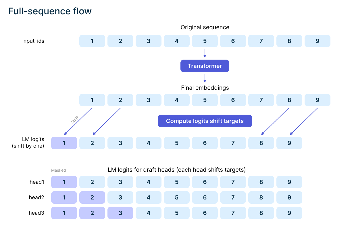
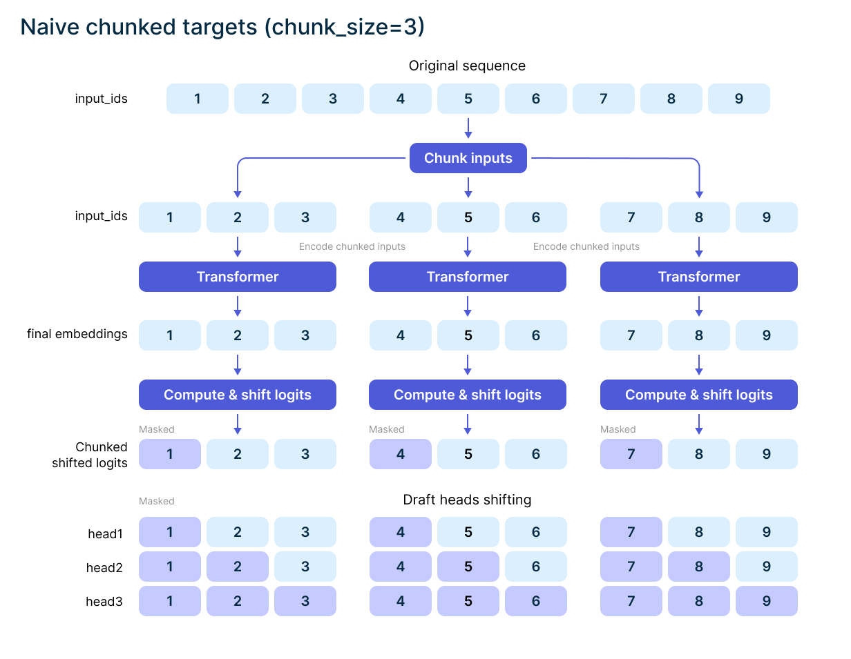
Here we see the draft-heads-shifting masks most of the boundary tokens as each head should rely on a previous token, but the previous token is stored in a previous chunk. Therefore, target shifting and mask alignment must happen before chunking.
Hidden states, targets, and masks are first transformed into the exact token-level objective, and only then split into chunks. This keeps Streaming Cross Entropy equivalent to dense Cross Entropy, except for small floating-point differences caused by reduction order.
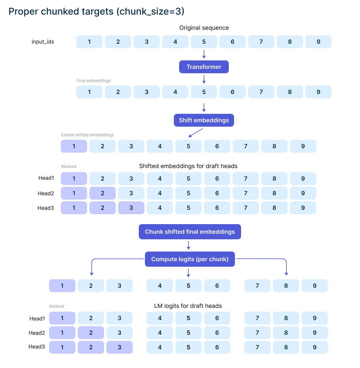
Backward pass
The forward pass computes the loss chunk by chunk. The backward pass follows the same idea. For each token chunk, we compute the local logits, Cross Entropy, and gradients. The input gradients are produced for the corresponding hidden-state chunk. The LM-head weight gradients are accumulated across chunks.
The production implementation wraps this logic in a custom backward rule, so the caller sees the same interface as a regular loss function while the implementation avoids storing the full logits tensor.
Conceptually:
for each token chunk:
    compute logits for the chunk
    compute chunk loss
    compute gradients for chunk hidden states
    compute gradient for LM-head
    accumulate gradients for LM-head weights
As a result, the peak memory is bounded by: chunk_size x vocab_size x dtype_size x 2.
For example, with:
chunk_size = 1024
vocab_size = 128k
dtype = fp32
the logits plus gradient buffer require: 1024 x 150_000 x 4 x 2 ~= 0.97GiB. Compare this with the dense example above, where the same path required hundreds of GiB.
This is conceptually similar to gradient accumulation, but the split happens inside the loss computation rather than across optimizer steps. We are not changing the training batch. We are changing how many token logits are materialized at one time.
Gradient accumulation reference:
, where mb — minibatch, n — number of minibatches in batch.
Streaming cross entropy loss:
The final loss must use the same normalization as the original dense objective. For token-level supervised fine-tuning, this usually means normalizing by the number of valid, non-masked tokens. It should not be normalized by the number of chunks.
Streaming Cross Entropy is orthogonal to the surrounding parallelism strategy. It can be used with FSDP, data parallelism, context parallelism, tensor parallelism, or no model parallelism at all. The technique only changes how many token logits are materialized locally at a time; it does not require changing the global training topology.
Choosing the chunk size
The chunk_size defines the maximum number of tokens for which logits are materialized at once. For example: chunk_size = 1024, means the largest logits tensor has shape: [1024, vocab_size] regardless of how those tokens are distributed across batch and sequence dimensions.
Lowering chunk_size reduces logits memory, but only up to a point. Once the LM loss path is no longer the peak memory consumer, making chunks smaller does not reduce the overall training peak. It only adds overhead: more loop iterations, more kernel launches, and less efficient matrix multiplications.
Therefore, the goal is not to make chunk_size as small as possible. The goal is to choose the largest chunk size that keeps the LM loss path below the next major memory peak in the training step. A useful heuristic is: streaming_lm_peak <= transformer_block_peak.
Once this condition holds, the LM loss path is no longer the dominant memory peak. Further reducing chunk_size mostly hurts performance without improving the actual peak memory of the compiled graph.
All runs have sequence_length=8192, batch_size=16, num_minibatches=2. After selecting chunk=X, sequence is split into n_chunks=Y; This picture clearly demonstrates performance degradation: increase of n_chunk significantly lowers performance due to overhead on iterations and inefficient matmuls on tiny subsequences.
Memory example (full finetuning)
Consider full fine-tuning of a Llama-3.1-8B-like model with:
Terminology:
-
dp — data parallel, number of independent data-executors.
-
cp — context parallel, shards sequence
-
microbatch size (it is effective batch size) equals
batch_size / (dp * gradient_accumulation)
context_length = 8192
microbatch_size = 4
dp = 2
cp = 1
FSDP enabled
activation dtype = bf16
logits dtype = fp32
During the forward pass, transformer block outputs are stored while most intermediate activations are rematerialized. Gradients are stored in fp32, master weights and optimizer states in fp32, and activations in bf16.
A rough memory estimate is:
Model state: 8B params × (fp32 weights + fp32 grads + 2 × fp32 optimizer states) / 2 devices ≈ 59 GB
Stored transformer block outputs: 32 layers × 4 × 8192 × 4096 × bf16 ≈ 8 GB
Dense Cross Entropy logits & gradient buffer: 4 x 8192 x 128k x fp32 x 2 = ~31GB
Streaming CE & gradient buffer with chunk_size=1024: 1024 x 128k x fp32 x 2 = ~1GB
So the rough estimate changes:
Dense CE: 59GB + 8GB + 31GB ~= 98GB
Streaming CE: 59GB + 8GB + 1GB ~= 68GB
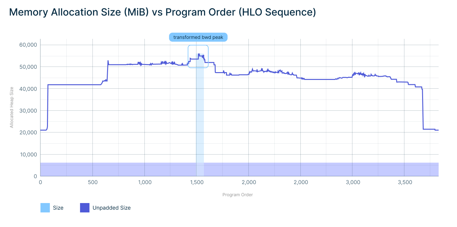
This does not necessarily mean that the compiled training graph will show a full 30 GB reduction in peak memory. Once the LM loss peak is removed, another part of the graph becomes the new peak.
Usually, the next significant peak is in the transformer block backward pass. To propagate gradients through a rematerialized transformer block, the training step has to recompute attention and MLP steps and store all the intermediate activations for the backward pass of a single block. Depending on the architecture, this peak may also include communication buffers or MoE-specific buffers. This is why chunk-size selection should be tied to the next-largest memory peak, not to an arbitrary minimum chunk size.
Why speculative decoding makes this more important
Speculative decoding training is similar to standard LM training: it still optimizes token-level prediction objectives. The difference is that it introduces one or more additional draft heads, such as EAGLE-style heads or MTP-style heads.
Each draft head predicts a future token. In the dense implementation, each head may produce its own logits tensor. In the worst case, the LM loss memory scales approximately as: num_heads × batch_size × sequence_length × vocab_size.
This makes the logits bottleneck much worse than in standard LM training. Streaming Cross Entropy applies naturally here. Each head’s token-level objective can be aligned, masked, chunked, and accumulated independently, without materializing full logits for all heads. The important detail is target shifting.
For draft head k, the target is shifted by k tokens. This shift must happen before chunking. Otherwise, a chunk boundary can split prediction-target pairs and produce an incorrect loss.
The correct order is:
for each draft head:
    align hidden states, targets, and masks
    split aligned tokens into chunks
    compute streaming Cross Entropy
    accumulate loss with correct scaling
This makes Streaming Cross Entropy especially useful for speculative decoding training: it removes a memory cost that would otherwise scale with the number of draft heads.
EAGLE 3 block-sparse masking for FlashAttention
Streaming Cross Entropy removes the vocabulary-logits bottleneck. For EAGLE 3 training, there is another bottleneck: the draft-head attention pattern itself.
EAGLE 3 draft-head training introduces sparse attention patterns that are not covered by a simple causal mask. Each token only needs to attend to a limited neighborhood relevant to the corresponding draft prediction. This creates a banded diagonal sparsity pattern.
A naive implementation may materialize or process much larger dense attention regions, which scales poorly with sequence length. This is especially problematic for long-context training, where dense attention memory grows quadratically with sequence length.
Attention kernels operate on fixed-size tiles, or blocks. Instead of materializing the full attention matrix of shape: [N, N] we can represent valid attention regions at block granularity. Blocks that intersect valid regions are computed. Blocks outside those regions are skipped.
For EAGLE 3, we extend this block-sparse masking mechanism to support draft-head diagonal bands. This composes with existing masking constraints:
causal masking
document packing
draft-head diagonal sparsity
In other words, the final block mask is the intersection of all constraints. A block is computed only if it is valid under the causal mask, the document-packing mask, and the draft-head sparsity pattern.
This allows EAGLE 3 training to reuse high-performance FlashAttention-style kernels instead of falling back to a dense or pure JAX implementation. The main benefit is both performance and memory efficiency.
The numbers below are implementation benchmarks for the tested configurations, not general product guarantees. They are useful because they show why the dense baseline becomes infeasible and why block-sparse attention matters for EAGLE 3 draft-head training.
Block-sparse attention benchmarks
For GPT-OSS-20B-like configurations with EAGLE 3 draft heads, block-sparse FlashAttention significantly outperforms the JAX baseline.
The benchmark below uses:
num_draft_tokens = 6
forward + backward
2 × H100 GPUs
Throughput (TFLOPS, FWD+BWD, num_draft_tokens=6, 2GPUs H100)
*Note: Triton TFLOPS is given as a range because later heads process more tokens that need diagonal masking
The JAX implementation scales quadratically with sequence length and quickly becomes infeasible. The block-sparse FlashAttention implementation scales much more favorably because invalid blocks are never materialized or processed.
For a full training run on a pod with 8 H100 GPUs with GPT-OSS-20B, we see a reduction in GPU memory utilization from 44% down to 25% and an increase of tokens per second from 6900 to 11200. As memory utilization lowered, we could increase effective batch_size to fully utilize gpu resources. Block-sparse attention is not just an optimization, it is an enabler for training EAGLE 3 draft heads at scale.
Memory example (speculator training)
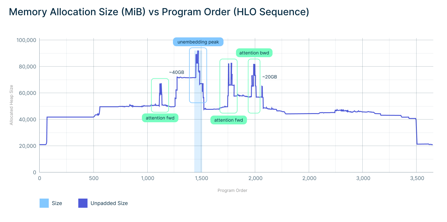
The memory profiles below show how these features affect a speculator-training run.
model: unsloth/gpt-oss-20b-BF16
context: 8k
dp=4, cp=1, bs=32, nmb=1 (tokens per gpu = 8 * 8192 = 65 536)
Eagle3 drafter, num decoding heads=3
Default attention + LM pass
Default attention + Streaming LM pass
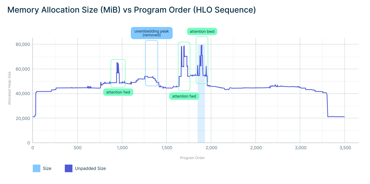
Eagle 3 sparse mask + LM pass
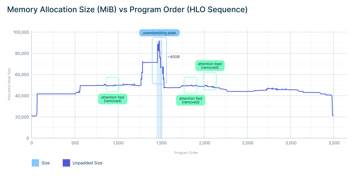
Eagle 3 sparse mask + Streaming LM pass
Conclusion
This page described two complementary techniques that target different bottlenecks in long-context LLM training with speculative draft heads.
Streaming Cross Entropy addresses the LM loss path. A dense implementation materializes a logits tensor of shape [batch_size, sequence_length, vocab_size], which can reach hundreds of GiB for realistic configurations — and scales further with the number of draft heads. Streaming Cross Entropy exploits the token-wise decomposability of the loss: it computes logits and Cross Entropy over small token chunks, accumulates the summed loss and gradients, and normalizes using the same denominator as the dense objective. The result is mathematically equivalent, with peak logits memory bounded by chunk_size × vocab_size × dtype_size × 2 regardless of the total token count.
Block-sparse FlashAttention addresses the draft-head attention pattern. EAGLE 3 introduces banded diagonal sparsity that a naive dense implementation would process at quadratic cost in sequence length. By representing valid attention regions at block granularity — intersecting causal, document-packing, and draft-head diagonal constraints — only the blocks that matter are computed. For GPT-OSS-20B-scale configurations, this reduces GPU memory utilization from 44% to 25% and increases throughput from 6 900 to 11 200 tokens per second.
The two techniques compose naturally. Streaming Cross Entropy removes the vocabulary-logits bottleneck; block-sparse attention removes the quadratic attention bottleneck. Together, they make large-scale long-context draft-head training feasible in both memory and throughput — supporting larger vocabularies, longer contexts, and multiple speculative heads without forcing either the LM loss or draft-head attention into infeasible memory regimes.
Want to train draft models for your own workload?
Custom Speculator Training is now live in Nebius Token Factory. If your workload has repeatable latency, throughput, or cost pressure, you can train workload-specific draft models from your own data and work with Nebius to evaluate them against real production traffic.
Talk to your SA about a spec decoding performance review
Explore Custom Speculator Training


Contents